Every once in a while, I dive into a topic in science for no reason other than that I find it interesting. This is how I learnt about Titan, laser-cooling, and random walks. This post is about the fourth topic in this series: solitons.

A soliton is a stable wave that maintains its shape and characteristics as it moves around. In 1834, a civil engineer named John Scott Russell spotted a single wave moving through the Edinburgh and Glasgow Union Canal in Scotland. He described it thus in a report to the British Association for the Advancement of Science in 1844 (pp. 319-320):

I was observing the motion of a boat which was rapidly drawn along a narrow channel by a pair of horses, when the boat suddenly stopped—not so the mass of water in the channel which it had put in motion; it accumulated round the prow of the vessel in a state of violent agitation, then suddenly leaving it behind, rolled forward with great velocity, assuming the form of a large solitary elevation, a rounded, smooth and well-defined heap of water, which continued its course along the channel apparently without change of form or diminution of speed. I followed it on horseback, and overtook it still rolling on at a rate of some eight or nine miles an hour [14 km/h], preserving its original figure some thirty feet [9 m] long and a foot to a foot and a half [30−45 cm] in height. Its height gradually diminished, and after a chase of one or two miles [2–3 km] I lost it in the windings of the channel.

Such, in the month of August 1834, was my first chance interview with that singular and beautiful phenomenon which I have called the Wave of Translation, a name which it now very generally bears; which I have since found to be an important element in almost every case of fluid resistance, and ascertained to be the type of that great moving elevation in the sea, which, with the regularity of a planet, ascends our rivers and rolls along our shores.

Russell was able to reproduce a similar wave in a water tank and study its properties. American physicists later called this wave a 'soliton' because of its solitary nature as well as to recall the name of particles like protons and electrons (to which waves are related by particle-wave duality).

Solitons are unusual in many ways. They are very stable, for one: Russell was able to follow his soliton for almost 3 km before it vanished completely. Solitons are able to collide with each other and still come away intact. There are types of solitons with still more peculiar properties.

These entities are not easy to find: they arise due to the confluence of unusual circumstances. For example, Russell's "wave of translation" was born when a boat moving in a canal suddenly stopped, pushing a single wave of in front that kept going. The top speed at which a wave can move on the surface of a water body is limited by the depth of the body. This is why a tsunami generated in the middle of the ocean can travel rapidly towards the shore, but as it gets closer and the water becomes shallower, it slows down. (Since it must also conserve energy, the kinetic energy it must shed goes into increasing its amplitude, so the tsunami becomes enormous when it strikes land.)

In fluid dynamics, the ratio of the speed of a vessel to the square root of the depth of the water it is moving in is called the Froude number. If the vessel was moving at the maximum speed of a wave in the Union Canal, the Froude number would have been 1.

If the Froude number had been 0.7, the vessel would have generated V-shaped pairs of waves about its prow, reminiscent of the common sight of a ship cutting through water.

Then the vessel started to speed up and its Froude number approached 1. This would have caused the waves generated off the sides to bend away from the prow and straighten at the front. This is the genesis of a soliton. Since the Union Canal has a fixed width, waves forming at the front of the vessel will have had fewer opportunities to dissipate and thus keep moving forward.

Since the boat stopped, it produced the single soliton that won Russell's attention. If it had kept moving, it would have produced a series of solitons in the water, and at the same have acquired a gentle up and down oscillating motion of its own as the Froude number exceeded 1.

Waves occur in a wide variety of contexts in the real world — and in the right conditions, scientists expect to find solitons in almost all of them. For example they have been spotted in optical fibres that carry light waves, in materials carrying a moving wave of magnetisation, and in water currents at the bottom of the ocean.

In the wave physics used to understand these various phenomena, a soliton is said to emerge as a solution to non-linear partial differential equations.

The behaviour of some systems can be described using partial differential equations. The plucked guitar string is a classic example. The string is fixed at both ends; when it is plucked, a wave travels along its length producing the characteristic sound. The corresponding equation goes like this: ∂²u/∂t² = c² • ∂u²/∂x², where u is the string's displacement, x is where it was plucked, c is the maximum speed the wave can have, and t is of course the time lapsed.

The equation itself is not important. The point is that there's a left-hand side and a right-hand side, and one side can equal the other for different combinations of u, x, and t. Each such combination is called a solution. One particular solution is called the soliton when the corresponding wave meets three conditions: it's localised, preserves its shape and speed, and doesn't lose energy when interacting with other solitons.

The "non-linear" part of "non-linear partial differential equations" means that these equations describe ways whose properties that have different properties depending on their amplitude. The guitar string equation is an example of a linear system because u, the string's displacement, has a power of 1 (i.e. it isn't squared or cubed) nor are the other terms of the equation multiplied with each other. Another famous example of a non-linear partial differential equation is the Schrödinger equation, which describes how the wave function of a quantum system will change over time given a set of initial conditions.

(The Austrian-Irish physicist Erwin Schrödinger postulated it in 1925, which is one of the reasons the UN has designated our current year — a century later — the International Year of Quantum Science & Technology.)

An example of a non-linear partial differential equation is the Korteweg-de Vries equation, which predicts how waves behave in shallow water: u_t + 6u • u_x + u_xxx = 0. The second term is the problem: u_x is a way to write ∂u/∂x and since it is multiplied by 6u the equation is non-linear, i.e. a change in its character induces changes in itself that may also change its character.

But for better or for worse, this is the only milieu in which a soliton will emerge.

(If you're really interested: for example a soliton solution of the Korteweg-de Vries equation looks like this: u = A sech² [ k (x – v_t – x₀​) ], where A is the soliton's amplitude or maximum height, k is a term related to its width, x₀ is its initial position, and v_t is its velocity over time. 'sech' is the hyperbolic secant function.)

Physicists are more interested in particular types of soliton than others because they closely mimic specific phenomena in the real world. Sometimes it's a good idea to understand these phenomena as if they were solitons because the mathematics of the latter may be easier to work with. This lucid Institute of Physics video starring theoretical physicist David Tong sets out the quirky case of quarks.

I myself was more piqued by the Peregrine and breather solitons.

The Peregrine soliton isn't a soliton that travels. Its name comes from its discoverer, a British mathematician named Howell Peregrine. In fact, one of the things that distinguish a Peregrine soliton is that it's stuck in one place. More specifically it emerges from pre-existing waves, has a much greater amplitude than the background, and appears at and disappears from a single location in a blip.

Peregrine solitons are interesting because they have been used to explain killer waves: freakish waves in the open sea that have no discernible cause and tower over all the other waves. One famous example is the Draupner wave, which was the first killer wave to also be measured by an instrument as it happened. It occurred on January 1, 1995, near the Draupner platform, a natural-gas rig in the Norwegian part of the North Sea. This is the wave's sounding chart:

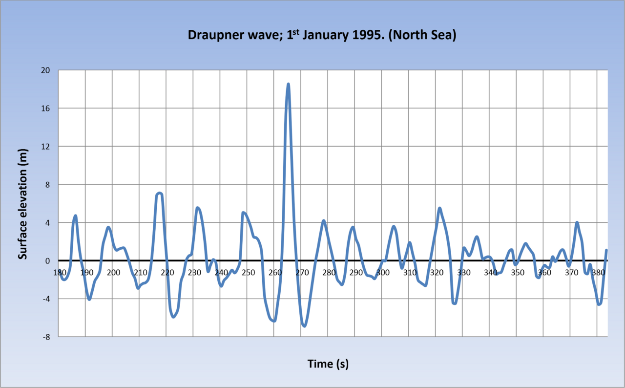
That's one heck of a soliton.

The breather soliton is equally remarkable. It's a regular soliton that also has an oscillating amplitude, frequency or something else as it moves around. Imagine a breather soliton to be a soliton in water: it might look like a wave with an undulating shape, its surface heaving one moment and sagging the other like the head of a strange sea monster breathing as it glides along. This is exactly the spirit in which the breathing soliton was named.

Here's an animation of a particular variety called the sine-Gordon breather soliton:

The Peregrine soliton is a particular instance of a breather soliton. Breathers have also been found in an exotic state of matter called a Bose-Einstein condensate (which physicists are studying with the expectation that it will inspire technologies of the future), in plasmas in outer space, in the operational parameters of short-pulse lasers, and in fibre optics. Some researchers also think entities analogous to breather solitons could help proteins inside the cells in our bodies transport energy.

If you're interested in jumping down this rabbit hole, you could also look up the Akhmediev and the Kuznetsov-Ma breathers.

At first blush, solitons seem like monastic wanderers of a world otherwise replete with waves travelling as if loath to be separated from another. Recall that one wave in 1834 gliding ever so placidly for over half a league, followed by a curious man on a horse galloping along the canal's bank. But for this venerable image, solitons are the children of a world far too sophisticated to admit waves crashing into each other with little more consequence than an enlivening spray of water and the formidable mathematics they demand to be understood.

Place a pot of water on the stove and light the fire. Once the temperature in the pot reaches 100º C or so, the water will boil to vapour. This is an example of a phase transition that occurs every day in our houses. Yet scientists have difficulty predicting whether a bunch of water molecules, like in the pot, will be liquid or gaseous in a given set of conditions.

This is different from your everyday experience with the pot on the stove and has to do with the model a computer can simulate to predict the phase of a group of interacting particles. Models that can make these predictions efficiently are prized in the study of wet surfaces, porous materials, microfluidics, and biological cells. They can also reveal ‘hidden’ phenomena we may not notice at the macroscopic level, i.e. just by looking at the water boil, and which scientists can use to make sense of other things and/or come up with new applications.

Remember your high school practicals notebook? For each experiment, you had to spell out sections called “given”, “to find”, “apparatus”, “methods”, and “results”. A model is an “apparatus” — a computer program — that uses the “given” (some input data) and certain “methods” (model parameters) to generate “results”. For example, the model below shows how a fluid with certain properties, like air, flowing around a spherical obstacle in its path, like a big rock, leads to the formation of vortices.

A popular “method” that models use to predict a phase transition is called classical density functional theory (DFT). Say there are a bunch of particles in a container. These particles can be the atoms of air, molecules of water, whatever the smallest unit of the substance is that you’re studying. Every three-dimensional distribution of these particles has a quantity called the free-energy functional associated with it. (Functionals and functions are the same thing except functionals can also accept functions as inputs.) The free-energy functional calculates the total free energy of a system based on how the density of its particles is distributed in three dimensions.

Classical DFT is a way to find the equilibrium state of a system — when it’s reached a stable state where its macroscopic properties don’t change and it doesn’t exchange energy with its surroundings — by minimising the system’s free energy.

A model can thus simulate a group of particles in a container, varying their distribution until it finds the one with the lowest free-energy functional, and thus the conditions in which the system is at its lowest energy. “Once [the free-energy functional] is specified, consistent and complete investigation of a wide variety of properties can be made,” the authors of a paper published in the journal Physical Review X on January 24 wrote.

While this sounds simple, the problem is that determining the free-energy functional becomes more difficult the more particles there are. And only once the functional has been determined can the model check when its value is lowest. This is why a model using classical DFT to determine the properties of a liquid at specific temperature and pressure, say, will struggle.

In the January 24 study in Physical Review X, scientists from the University of Bayreuth and the University of Bristol made an advance in this process when they replaced the free-energy functional with a neural network that had been trained on simulations of particles-in-a-container in a variety of conditions (e.g. changing the pressure and temperature across a range of values), then used it to model a realistic fluid.

From the abstract of the paper:

Local learning of the one-body direct correlation functional is based on Monte Carlo simulations of inhomogeneous systems with randomized thermodynamic conditions, randomized planar shapes of the external potential, and randomized box sizes.

Monte Carlo simulations are quite cool. You set up a computer to simulate, say, a poker game with five players. As the game progresses, at some point in the game you ask the computer to take a snapshot of the game and save it. This snapshot has information about each player’s cards, what decisions they made in the previous round (fold, call or raise), the stakes, and the cards on the table. Once the game ends, you rerun the simulation, each time freshly randomising the cards handed out to the players. Then again at some point during the game, the computer takes a snapshot and saves it.

Once the computer has done this a few thousand times, you collect all the snapshots and share them with someone who doesn’t know poker. Based on understanding just the snapshots, they can learn how the game works. The more snapshots there are, the finer their understanding will be. Very simply speaking this is how a Monte Carlo simulation operates.

The researchers generated data for the neural network to train on by running around 900 Monte Carlo simulations of “inhomogeneous systems with randomized thermodynamic conditions [including temperature], randomized planar shapes of the external potential, and randomized box sizes”. (The external potential refers to some energy field applied across the system, giving each of the particles inside some potential energy.) Then they used their classical DFT model with the “neural functional” to study a truncated Lennard-Jones system.

Scientists have previously combined machine-learning with classical DFT models to study particles moving randomly, interacting with each other only when they collide. Actual, real fluids aren’t so simple, however. Instead, their behaviour is more closely modelled as a Lennard-Jones system: the particles in a container repel each other at very short distances, are attracted to each other across intermediate distances, and at larger distances don’t have an effect on each other. As the researchers wrote in their paper:

… understanding the physics in such a simple model, which encompasses both repulsive and attractive interparticle interactions, provides a basis for understanding the occurrence of the same phenomena that arise in more complex fluids .

They also added that:

… recent investigations did not address the fundamental issue of how the presence of a phase transition might be accounted for within the framework of a neural density functional.

So they set about studying a truncated Lennard-Jones system with a phase transition. Their model started with predicting how the particles are distributed, the overall system’s thermodynamic properties, the conditions in which liquid and gaseous phases coexist in the container, and the particles’ behaviour at interfaces, like evaporating from the surface of a hard wall. Then, the researchers wrote:

… we focus on the liquid-gas transition which is a basic manifestation of the presence of interparticle attraction and seek to assess whether the neural functional can describe (i) phase coexistence and the approach to the associated critical point, (ii) surface tension and density profiles of the liquid-gas interface, (iii) drying and capillary evaporation transitions that occur at subcritical temperatures, and (iv) how accurately the approach performs for both bulk and interfacial properties.

(Emphasis in the original.)

So could the neural functional describe i-iv?

The answer is emphatically yes.

In fact, the model was able to accurately predict phase transitions even when it was trained only on supercritical states — i.e. when the container contains both liquid and gaseous states. The researchers singled this ability of the model out for especial praise, calling it “one of the most striking results”.

This plot, generated by the model, shows the states of a truncated Lennard-Jones fluid with density on the x-axis and temperature on the y-axis. In the red areas, the substance — the collection of particles in the box — is either liquid or gaseous. In the blue areas, the liquid and gaseous phases become separated. The intensity of the colour denotes the substance’s bulk modulus, i.e. how much it resists being compressed at a fixed temperature, from dark blue at the lower end to dark red at the upper.

Overall, the researchers wrote their “neural functional approach” is distinguished by the fact that “the range of phenomena and results it can describe … far exceed the information provided during training.” They attribute this ability to the information contained in a “single numerical object” that the neural network was tuned to track: 𝑐1⁡(𝐫;[𝜌],𝑇), a.k.a. the one-body direct correlation functional. It’s a functional that describes the variation of the density of particles inside the container in response to the external potential. As they put it:

Inputting only Monte Carlo training data of one-body profiles in planar geometry and then examining 𝑐1⁡(𝐫;[𝜌],𝑇) through the functional lens provides access to quantities which could not be obtained directly from the input data. Indeed, determining these usually requires advanced simulation techniques.

They added their method also required fewer computational resources than a classical DFT setup operating without a neural functional in order to achieve “comparable” accuracy. On the back of this resounding success, the researchers plan to use their model to study interactions in water and colloidal gels. They also wrote that they expect their findings will help solve problems in computational chemistry and condensed matter physics.